Algorithms
This package implements four different algorithms to solve the two-satge minimum wright spanning tree problem.
Random instances for the problem can be generated as follows:
using TwoStageSpanningTree, BenchmarkTools
n = 5
m = 4
instance = TwoStageSpanningTreeInstance(; n, m, nb_scenarios=20, seed=0);
1. Cut generation algorithm
As presented in the problem statement, the MIP formulation of the minimum weight two-stage spanning tree problem has an exponential number of constraints. We cannot solve it directly using a MIP solver, but we can solve it with a subset of constraints and iteratively add the most violated one, up until all constraint are satisfied.
Finding the most violated constraint (for a given scenario $s$) is called the separation problem, and can be formulated as:
\[\begin{aligned} \min_Y\quad & |Y| - 1 - \sum_{e\in E(Y)}(y_e + z_{es})\\ \text{s.t.}\quad & \emptyset \subsetneq Y\subsetneq V \end{aligned}\]
with $y$, $z$ fixed and obtained by minimizing the problem restricted to a subset of constraints.
If the value of this problem is positive for all scenarios, then all constraints are satisfied and the optimal solution is found.
MIP separation problem
A straightforward way to solve the separation problem, is to formulate it as the following MILP:
\[\begin{array}{rll} \min\limits_{\alpha, \beta}\, & \sum\limits_{v\in V}\alpha_v - 1 - \sum\limits_{e \in E} \beta_e (y_e + z_{es}) \\ \mathrm{s.t.}\, & 2 \beta_{e} \leq \alpha_u + \alpha_v \qquad & \forall e = (u,v)\in E \\ & \sum\limits_{v\in V} \alpha_v \geq 1\\ & \alpha, \beta \in \{0,1\} \end{array}\]
This separation solver is implemented as MILP_separation_problem and can be given as input option to the cut_generation method:
mip_solution = cut_generation(instance; separation_problem=MILP_separation_problem)TwoStageSpanningTreeSolution(Bool[0, 0, 0, 0, 0, 1, 0, 1, 0, 0 … 0, 1, 0, 1, 0, 0, 1, 1, 1, 0], Bool[0 0 … 1 1; 1 1 … 0 1; … ; 0 0 … 0 0; 0 1 … 1 1])The solution feasibility can be tested with the is_feasible method:
is_feasible(mip_solution, instance)trueThe objective value of a given solution can be computed using the solution_value method:
solution_value(mip_solution, instance)83.3Solutions can be visualized scenario by scenario using the plot_scenario method:
plot_scenario(mip_solution, instance, 1; n, m)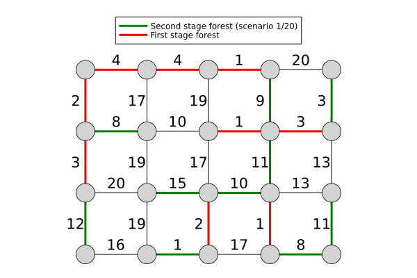
Cut separation problem
The separation problem can alternatively be formulated as a min-cut problem, which has better performance and scaling.
The separation problem
\[\min |Y| - 1 - \sum_{e \in E(Y)} (y_e + z_{es}) \quad \text{subject to} \quad \emptyset \subsetneq Y \subsetneq V\]
is equivalent to
\[\min |Y| + \sum_{e \notin E(Y)} (y_e + z_{es}) - |V| \quad \text{subject to} \quad \emptyset \subsetneq Y \subsetneq V.\]
Let us define the digraph $\mathcal{D} = (\mathcal{V}, \mathcal{A})$ with vertex set $\mathcal{V} = \{s,t\} \cup V \cup E$ and the following arcs.
| Arc $a$ | Capacity $u_a$ |
|---|---|
| $(s,e)$ for $e \in E$ | $y_e + z_{es}$ |
| $(e,u)$ and $(e,v)$ for $e = (u,v) \in E$ | $+\infty$ |
| $(v,t)$ for $v \in V$ | $1$ |
The separation problem is equivalent to finding a non-empty minimum-capacity $s$-$t$ cut $Y$ in $\mathcal{D}$. This can be done with the following MILP:
\[\begin{array}{rll} \min \, & \sum\limits_{a \in \mathcal{A}} u_a \beta_a \\ \mathrm{s.t.} \, & \alpha_s - \alpha_t \geq 1 \\ & \beta_a \geq \alpha_u - \alpha_v & \text{ for all } a= (u,v) \in \mathcal{A} \\ & \sum\limits_{v \in V} \alpha_v \geq 1 \\ & \alpha, \beta \in \{0,1\} \end{array}\]
This separation solving method is implemented by cut_separation_problem and is also compatible with cut_generation.
We observe that using it is faster than the other method.
cut_solution = cut_generation(instance; separation_problem=cut_separation_problem)TwoStageSpanningTreeSolution(Bool[0, 0, 0, 0, 0, 1, 0, 1, 0, 0 … 0, 1, 0, 1, 0, 0, 1, 1, 1, 0], Bool[0 0 … 1 1; 1 1 … 0 1; … ; 0 0 … 0 0; 0 1 … 1 1])@benchmark cut_generation(instance; separation_problem=MILP_separation_problem)BenchmarkTools.Trial: 1 sample with 1 evaluation.
Single result which took 141.976 s (0.10% GC) to evaluate,
with a memory estimate of 1.98 GiB, over 75237358 allocations.@benchmark cut_generation(instance; separation_problem=cut_separation_problem)BenchmarkTools.Trial: 1 sample with 1 evaluation.
Single result which took 14.253 s (0.78% GC) to evaluate,
with a memory estimate of 1.35 GiB, over 27728437 allocations.is_feasible(cut_solution, instance)truesolution_value(cut_solution, instance)83.32. Column generation
Since minimum spanning tree can be solved efficiently, it is natural to perform a Dantzig-Wolfe reformulation of the problem previously introduced.
It leads to the following formulation.
\[ \begin{array}{rll} \min\,& \displaystyle\sum_{e \in E}c_e y_e + \frac{1}{|S|}\sum_{e \in E}\sum_{s \in S}d_{es}z_{es}\\ \mathrm{s.t.} \,& y_e + z_{es} = \displaystyle\sum_{T \in \mathcal{T}\colon e \in T} \lambda_{T}^s & \text{for all $e\in E$ and $s \in S$} \\ & \displaystyle\sum_{T \in \mathcal{T}} \lambda_{T}^s = 1 & \text{for all }s \in S \\ & y,z,\lambda\in \{0,1\} \end{array}\]
The linear relaxation of this problem can be solved by column generation, and the problem itself can be solved using a Branch-and-Price. The linear relaxation is implemented by column_generation, and an heuristic using columns outputed by it is implemented by column_heuristic:
column_solution = column_heuristic(instance)TwoStageSpanningTreeSolution(Bool[0, 0, 0, 0, 0, 1, 0, 1, 0, 0 … 0, 1, 0, 1, 0, 0, 1, 1, 1, 0], Bool[0 0 … 1 1; 1 1 … 0 1; … ; 0 0 … 0 0; 0 1 … 1 1])@benchmark column_heuristic(instance)BenchmarkTools.Trial: 2 samples with 1 evaluation.
Range (min … max): 3.190 s … 3.210 s ┊ GC (min … max): 0.06% … 0.07%
Time (median): 3.200 s ┊ GC (median): 0.07%
Time (mean ± σ): 3.200 s ± 14.078 ms ┊ GC (mean ± σ): 0.07% ± 0.01%
█ █
█▁▁▁▁▁▁▁▁▁▁▁▁▁▁▁▁▁▁▁▁▁▁▁▁▁▁▁▁▁▁▁▁▁▁▁▁▁▁▁▁▁▁▁▁▁▁▁▁▁▁▁▁▁▁▁█ ▁
3.19 s Histogram: frequency by time 3.21 s <
Memory estimate: 65.07 MiB, allocs estimate: 370821.is_feasible(column_solution, instance)truesolution_value(column_solution, instance)83.33. Benders decomposition
The integer optimal solution of the column generation formulation can be found using a Branch-and-price, quite heavy to implement. Another option is to apply a Benders decomposition to decouple the scenarios.
When first stage variables $y$ are fixed, the subproblem for scenario $s$ becomes:
\[\begin{aligned} \min_{z, \lambda}\quad & \sum_{e\in E}d_{es} z_{es}\\ \text{s.t.}\quad & z_{es} = \sum_{T\in \mathcal{T}\colon e\in T}\lambda_T^s - y_e & \forall e \in E\\ & \sum_{T\in\mathcal{T}}\lambda_T^s = 1\\ & z, \lambda\geq 0 \end{aligned}\]
We can simplify further the formulation by removing variable $z$:
\[\begin{aligned} \min_{z, \lambda}\quad & \sum_{T\in\mathcal{T}}\sum_{e\in T}d_{es}\lambda_T^s - cst(y_e) \\ \text{s.t.}\quad & \sum_{T\in \mathcal{T}\colon e\in T}\lambda_T^s \geq y_e & \forall e \in E\\ & \sum_{T\in\mathcal{T}}\lambda_T^s = 1\\ & z, \lambda\geq 0 \end{aligned}\]
We take its dual:
\[\begin{aligned} \max_{\mu, \nu}\quad & \nu_s + \sum_{e\in E} y_e \mu_{es} - cst \\ \text{s.t.}\quad & \sum_{e\in T} (d_{es} - \mu_{es}) - \nu_s \geq 0, & \forall T\in\mathcal{T}\\ & \mu\geq 0, \nu\in\mathbb{R} \end{aligned}\]
This dual can be solved using constraint generation, with once again a usual minimum spanning tree separation problem that can be solved using Kruskal algorithm:
\[\min \sum_{e\in T} (d_{es} - \mu_{es})\]
If the primal is feasible, we generate an optimality cut:
\[\theta_s \geq \nu_s + \sum_{e\in E} \mu_{es}y_e - \sum_{e\in E} d_{es} y_e\]
When the primal is unfeasible, there is an unbounded ray for the dual, i.e. $\mu, \nu$ such that $\nu_s + \sum_e \mu_{es} y_e > 0$ and $-\nu_s - \sum_{e\in T}\mu_{es}$. ($\alpha \nu$ and $\alpha\mu$ are also solutions for all $\alpha > 0$). Such solution can be found by solving:
\[\begin{aligned} \max_{\mu, \nu}\quad & \nu_s + \sum_{e\in E} \mu_{es} y_e \\ \text{s.t.}\quad & -\nu_s - \sum_{e\in T}\mu_{es} \geq 0 & \forall T\in \mathcal{T}\\ & 0 \leq \mu_{es} \leq 1 & \forall e\in E\\ & \nu_s\leq 1 \end{aligned}\]
Let us denote $\mathcal{F}$ the feasibility cuts and $\mathcal{O}_s$ the optimality cuts set. We obtain the following Benders master problem:
\[\begin{aligned} \max_{y}\quad & \sum_{e\in E} c_e y_e + \frac{1}{|S|}\sum_{s\in S}\theta_s \\ \text{s.t.}\quad & \theta_s \geq \nu_s + \sum_{e\in E} \mu_{es} y_e - \sum_{e\in E} d_{es} y_e & \forall s\in S,\, \forall (\nu, \mu) \in \mathcal{O}_s\\ & \nu + \sum_{e\in E} \mu_e y_e & \forall (\nu, \mu)\in \mathcal{F}\\ & y\in\{0, 1\} \end{aligned}\]
The benders_decomposition implements this method:
benders_solution = benders_decomposition(instance)TwoStageSpanningTreeSolution(Bool[0, 0, 0, 0, 0, 1, 0, 1, 0, 0 … 0, 1, 0, 1, 0, 0, 1, 1, 1, 0], Bool[0 0 … 1 1; 1 1 … 0 1; … ; 0 0 … 0 0; 0 1 … 1 1])@benchmark benders_decomposition(instance)BenchmarkTools.Trial: 3 samples with 1 evaluation.
Range (min … max): 2.243 s … 2.248 s ┊ GC (min … max): 3.61% … 3.97%
Time (median): 2.244 s ┊ GC (median): 3.84%
Time (mean ± σ): 2.245 s ± 2.859 ms ┊ GC (mean ± σ): 3.81% ± 0.18%
█ █ █
█▁▁▁▁▁▁▁▁▁▁▁▁▁▁▁▁█▁▁▁▁▁▁▁▁▁▁▁▁▁▁▁▁▁▁▁▁▁▁▁▁▁▁▁▁▁▁▁▁▁▁▁▁▁█ ▁
2.24 s Histogram: frequency by time 2.25 s <
Memory estimate: 860.88 MiB, allocs estimate: 17250205.is_feasible(benders_solution, instance)truesolution_value(benders_solution, instance)83.34. Lagrangian relaxation
Let us introduce one copy of first stage variables $y$ per scenario. An equivalent formulation of the problem is
\[\begin{array}{ll} \min\, & \displaystyle \sum_{e\in E}c_e y_e + \sum_{e \in E} \sum_{s \in S}d_{es}z_{es} \\ \mathrm{s.t.}\, & \mathbf{y}_s + \mathbf{z}_s \in \mathcal{P}, \quad\quad \text{for all $s$ in $S$} \\ & y_{es} = y_e, \quad \quad \quad \,\text{for all $e$ in $E$ and $s$ in $S$} \end{array}\]
Let us relax (dualize) the constraint $y_{es} = y_e$. We denote by $\theta_{es}$ the associated Lagrange multiplier.
The Lagrangian dual problem becomes
\[\begin{array}{rlrlrl} \max_{\theta}\mathcal{G}(\theta)= \min_{y}& \sum_{e \in E}(c_e + \frac{1}{|S|}\sum_{s \in S} \theta_{es})y_e \\ &+ \frac{1}{|S|}\sum_{s \in S}\min_{\mathbf{y}_s,\mathbf{z}_s} \sum_{e \in E}d_{es}z_{es} - \theta_{es}y_{es}\\ \mathrm{s.t.} & 0 \leq \mathbf{y} \leq M\\ & \mathbf{y}_s + \mathbf{z}_s \in \mathcal{P}, \quad\quad \text{for all $s$ in $S$} \end{array}\]
where $M$ is a large constant. In theory, we would take $M=+\infty$, but taking a finite $M$ leads to more informative gradients.
We have
\[(\nabla \mathcal{G}(\theta))_{es}= \frac{1}{|S|} (y_e - y_{es}).\]
Considering the sum on the second stage scenarios as an expectation, we can get stochastic gradients and maximize $\mathcal{G}$ using gradient ascent.
Once a solution of the relaxed problem is found, we have one solution $y_s$ per scenario $s$. We can then use an heuristic to reconstruct a good first stage decision $y$.
The lagrangian_relaxation method implements this heuristic:
solution, (; ub_history, lb_history) = lagrangian_relaxation(instance; nb_epochs=25000)(TwoStageSpanningTreeSolution(Bool[0, 0, 0, 0, 0, 1, 0, 1, 0, 0 … 0, 1, 0, 1, 0, 0, 1, 1, 1, 0], Bool[0 0 … 1 1; 1 1 … 0 1; … ; 0 0 … 0 0; 0 1 … 1 1]), (lb = 83.0976138937488, ub = 83.3, best_theta = [-12.006932482972793 -15.007348088496224 … -13.006219386699618 -7.006453798809543; -12.006901067883822 -15.005898389939647 … -13.00760072106909 -7.007835739530329; … ; -0.9998971735509196 -0.9998971735509196 … -0.9998971735509196 -0.9998971735509196; -9.003327130863028 -2.0067862263899836 … -7.007335814637157 -3.0059434343710345], lb_history = [0.0, 0.006999998600000279, 0.020949986145160637, 0.03633246164080159, 0.05248061480149503, 0.06758024632766592, 0.08210482635979983, 0.09590500828604871, 0.11048415084952032, 0.12608030884224528 … 83.09411315910612, 83.09460627462344, 83.09496415021687, 83.09533038133962, 83.09559216959877, 83.0959608410161, 83.0965045532183, 83.09493249360916, 83.0976138937488, 83.09567396785975], ub_history = [202.0, 202.0, 202.0, 202.0, 202.0, 202.0, 202.0, 202.0, 202.0, 202.0 … 83.3, 83.3, 83.3, 83.3, 83.3, 83.3, 83.3, 83.3, 83.3, 83.3]))@benchmark lagrangian_relaxation(instance; nb_epochs=25000)BenchmarkTools.Trial: 4 samples with 1 evaluation.
Range (min … max): 1.399 s … 1.410 s ┊ GC (min … max): 2.69% … 2.61%
Time (median): 1.404 s ┊ GC (median): 2.71%
Time (mean ± σ): 1.404 s ± 4.432 ms ┊ GC (mean ± σ): 2.71% ± 0.07%
█ █ █ █
█▁▁▁▁▁▁▁▁▁▁▁▁▁▁▁▁▁▁▁▁▁▁▁▁▁█▁▁▁▁█▁▁▁▁▁▁▁▁▁▁▁▁▁▁▁▁▁▁▁▁▁▁▁█ ▁
1.4 s Histogram: frequency by time 1.41 s <
Memory estimate: 2.70 GiB, allocs estimate: 10519518.is_feasible(benders_solution, instance)truesolution_value(benders_solution, instance)83.3We can plot the evolution of both lower and upper bounds along iterations
using Plots
f = plot()
plot!(f, ub_history; label="Upper bound: lagrangian heuristic", color=:orange)
plot!(f, lb_history; label="Lower bound: lagrangian relaxation", color=:purple)
f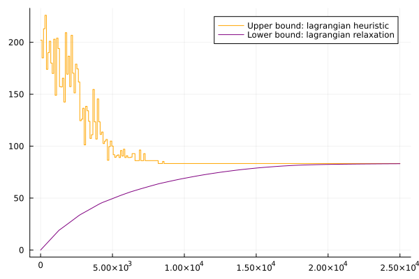
This page was generated using Literate.jl.